Introduction
In machine learning, we divide data used for model preparation into distinct groups.
A model cannot be developed on a dataset and then evaluated on the same data used to train it, as this would lead to biased and unreliable results. This is because the model would have already been exposed to and learned from the data during its development phase. Consequently, when evaluated on the same data, it would appear to perform exceptionally well, giving a false impression of its true capabilities.
Overfitting occurs because the model has memorized the training data rather than learning generalizable patterns. As a result, the model’s performance on this familiar data would not accurately reflect its ability to make predictions or classifications on new, unseen data, which is the ultimate goal of machine learning.
Dataset division in Machine Learning
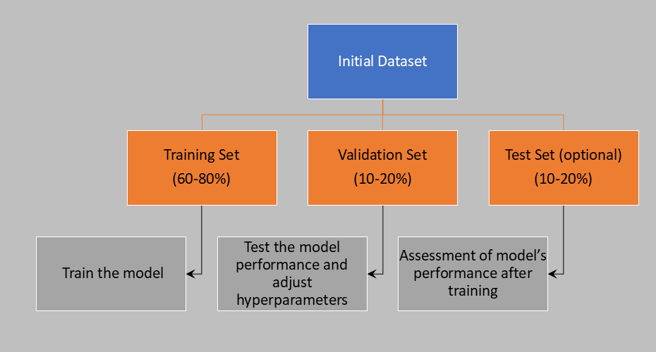
Typically, we divide the data sample into three groups:
Training set: This is generally the largest portion of the data (60-80%), used to train the model.
Validation set: This is used to test the model’s performance and adjust hyperparameters, helping to improve the model’s ability to generalize. It comprises 10-20% of the data.
Test set: This is used after training to evaluate the model’s performance. It provides an unbiased assessment of the model’s functionality and ability to generalize. In this case as well, 10-20% of the total data is included in the test group.

Sometimes, the data is divided into only two groups—training set and test set—without using a validation set.
The methods of dataset division vary and depend on both the dataset’s composition and the model’s objective.
The most commonly applied methods are:
Random Split: Divides the dataset into groups randomly.
Stratified Split: A classification method that maintains the proportion of classes across groups, ensuring uniform representation.
Time-based Split: Trains the model on past data and validates it on future data, used for temporal datasets.
In certain contexts, particularly in the medical field, datasets can be imbalanced. To address this issue, it’s often necessary to employ oversampling or undersampling techniques. These methods ensure that all classes within the dataset are uniformly represented, leading to more accurate and reliable model performance.
Scikit-learn, a popular Python library, aids in dataset division by providing widely used methods such as train_test_split and StratifiedShuffleSplit.
Simple division with train_test_split
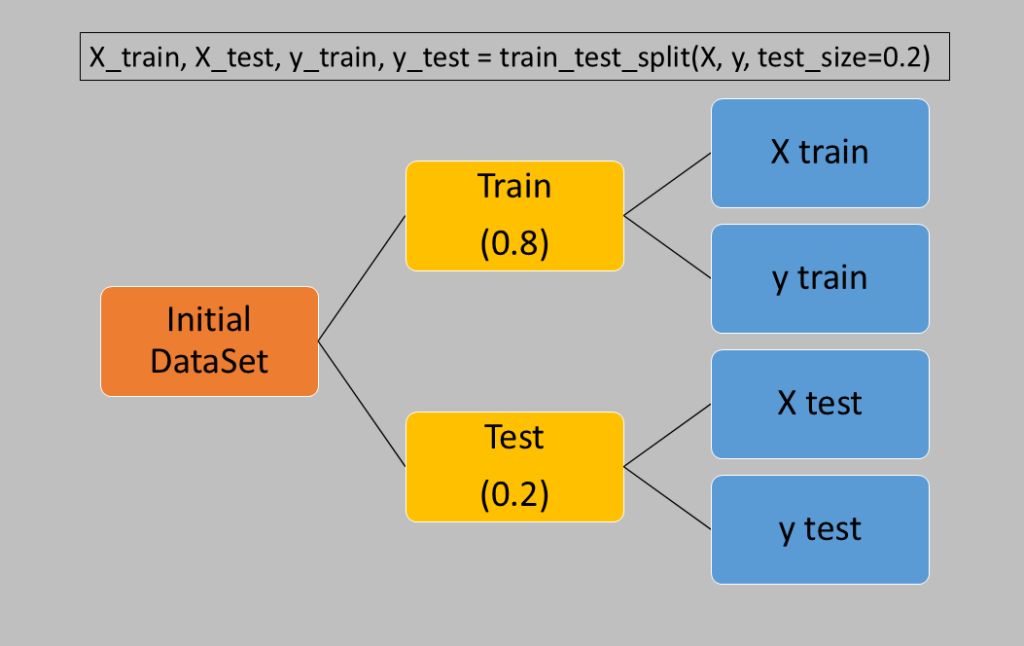
The train_test_split function of scikit-learn provides four variables that contain distinct segments of the dataset:
X_train: samples used for training
X_test: samples used for testing
y_train: outputs (targets) of the samples used for training
y_test: outputs (targets) of the samples used for testing
The ratio between the test and training samples is specified by the test_size parameter, which accepts values from 0 (no elements extracted for testing) to 1 (all elements used for testing). Typically, this parameter is set to 0.2, meaning 20% of the dataset elements are included in the test group.

Syntactically, it’s used as follows:
from sklearn.model_selection import train_test_split
import numpy as np

# Creating sample data
X = np.random.rand(100, 5)  # 100 samples, 5 features
y = np.random.randint(0, 2, 100)  # 100 binary class labels

# Splitting into training set (80%) and test set (20%)
X_train, X_test, y_train, y_test = train_test_split(X, y, test_size=0.2, random_state=42)
If we need a validation set as well, we can apply the train_test_split function a second time to the training data obtained from the first split. This allows us to extract an additional portion to be used as validation data:
# First division: 80% training + validation, 20% test
X_train_val, X_test, y_train_val, y_test = train_test_split(X, y, test_size=0.2, random_state=42)

# Second division: 20% validation, 80% training
X_train, X_val, y_train, y_val = train_test_split(X_train_val, y_train_val, test_size=0.25, random_state=42)
Stratified division with StratifiedShuffleSplit
In medical datasets, it’s common to encounter categorical variables where one class is significantly underrepresented compared to others. For instance, consider the dependent variable related to the comorbidity “renal insufficiency” in a dataset of patients with cardiac pathology. Despite being a crucial comorbidity that cannot be overlooked, the percentage of people affected by it may be considerably lower than those who are not.
This scenario leads to a phenomenon known as dataset imbalance.
A well-balanced dataset is one in which all classes are represented equitably. However, perfect balance is often unattainable in real-world scenarios, especially in medical data. The imbalance can significantly impact model performance, as algorithms favor the majority class, potentially leading to poor predictions for the minority class.
We’ll address methods for resolving this problem elsewhere. Our focus here is on handling situations where a class is underrepresented, ensuring that the minority variable is proportionally represented across the various dataset segments created for training and testing the machine learning model.
Scikit-learn’s StratifiedShuffleSplit function helps maintain class proportions during dataset division.
from sklearn.model_selection import StratifiedShuffleSplit

strat_split = StratifiedShuffleSplit(n_splits=1, test_size=0.2, random_state=42)
for train_index, test_index in strat_split.split(X, y):
    X_train, X_test = X[train_index], X[test_index]
    y_train, y_test = y[train_index], y[test_index]
Division with K-fold
We can divide our original dataset into k parts and train the model using each of these subsets. This approach is known as k-fold cross-validation.
Scikit-learn provides the KFold function for this type of division. If we want to maintain the class composition as in the previous case, we can use StratifiedKFold instead.
from sklearn.model_selection import KFold

kf = KFold(n_splits=5, shuffle=True, random_state=42)

for train_index, test_index in kf.split(X):
    X_train, X_test = X[train_index], X[test_index]
    y_train, y_test = y[train_index], y[test_index]
    # Train and evaluate the model for each fold

# Stratified K Fold:

from sklearn.model_selection import StratifiedKFold

skf = StratifiedKFold(n_splits=5, shuffle=True, random_state=42)

for train_index, test_index in skf.split(X, y):
    X_train, X_test = X[train_index], X[test_index]
    y_train, y_test = y[train_index], y[test_index]
    # Train and evaluate the model for each fold
The process works as follows:
Division into k folds: Initially, the dataset is divided into k equal parts. For example, with a dataset of 100 samples and k=5, we get 5 subsets of 20 samples each.
Training and testing iterations: For each iteration, one of the folds is chosen as the test set, and the remaining k-1 folds are used as the training set. This means that in each iteration we use:
- 1 fold for the test set (which varies with each iteration).
- The other k-1 folds for training (the rest of the dataset minus the test fold).
Repetition k times: The process is repeated k times, changing the fold used as the test set each time. This way, each sample in the dataset is used exactly once for testing and k-1 times for training.
Aggregation of results: At the end, performance metrics (such as accuracy, precision, etc.) are calculated for each iteration and averaged, obtaining an overall evaluation.
The diagram illustrates how data is divided into K folds, showing which portions are used for training versus testing during each iteration (using 20 samples and k=5).

Temporal division with TimeSeriesSplit
For time series data, TimeSeriesSplit allows us to divide the dataset into a training set using older data and a test set using more recent data.
from sklearn.model_selection import TimeSeriesSplit

tscv = TimeSeriesSplit(n_splits=5)

for train_index, test_index in tscv.split(X):
    X_train, X_test = X[train_index], X[test_index]
    y_train, y_test = y[train_index], y[test_index]
    # Train and evaluate the model for each temporal division
In this case, the function divides the sets chronologically, assuming they’re already arranged in time order. It’s the responsibility of those preparing the dataset to ensure the data is correctly sequenced.
Other types of divisions
The ShuffleSplit function is useful for creating multiple random divisions to generate additional training/test sets, particularly beneficial for large datasets.
For datasets derived from distinct groups (such as different patient cohorts), GroupKFold allows us to create training/test sets that contain members from only one group, effectively creating separate sets for each group.
Data leakage in Machine Learning
The Machine Learning model we’ve chosen undergoes a learning phase using the training data obtained from the initial dataset. We then evaluate its performance with the test dataset.
Crucially, the training dataset should have no overlap with the test set. If there’s commonality, the model might perform well not because it’s making accurate predictions, but because it’s simply recalling examples it has already seen.
This scenario leads to an overestimation of the model’s performance—a misleading outcome. When the model is deployed in production and encounters entirely new data, it might unexpectedly exhibit poor predictive ability, despite its seemingly good performance on the test set.
It’s akin to giving students exam questions in advance. Everyone would ace the test, but if it were repeated with unfamiliar questions, the results could be dramatically different.
This phenomenon is known as “data leakage.”
Data leakage can occur at two levels: train-test and target. Train-test leakage happens when a feature is calculated using the entire dataset, inadvertently influencing the test set with information it shouldn’t have. Target leakage occurs when a variable contains information related to the target that the model shouldn’t access.
Consider a train-test leakage example: we’re developing a model to predict house prices. Our target is “price,” with variables like “area,” “number_of_rooms,” and “age_of_house.” If we normalize the data before splitting it into train and test sets, we’ll use means and standard deviations from the entire dataset. This process introduces information into the test set that it shouldn’t have, compromising the model’s evaluation.
For target-level leakage, imagine a model predicting whether a debtor will repay a loan on time. The target variable is “payment_on_time,” with predictors like “age,” “income,” and “employment_status.” Including “account_balance” at the time of expected payment introduces leakage. This variable directly influences the ability to pay on time—if the balance is less than the amount due, it indirectly indicates non-payment. By incorporating future information, we make the model unreliable for real-world predictions.
To prevent data leakage, it’s crucial to follow these key steps:
Early Dataset Division: Split your data into training and test sets before any transformations
Isolated Transformations: Apply changes only to training data, then use those parameters for test data
Proper Validation: Implement suitable cross-validation techniques
Careful Feature Selection: Exclude variables that contain future information or are too closely related to the target variable
Further Reading
Leakage (machine learning) – Wikipedia
Summary and Conclusion
In conclusion, proper dataset division and prevention of data leakage represent fundamental elements for developing robust and reliable machine learning models. We have explored various data division methodologies, from the simplest like random split to more complex ones like k-fold cross-validation, highlighting the importance of choosing the most suitable approach based on dataset characteristics and model objectives. Particular attention must be paid to managing imbalanced datasets, especially in the medical field, where fair representation of minority classes is crucial for predictive accuracy.
Furthermore, we have analyzed the phenomenon of data leakage in its various forms, emphasizing how it can seriously compromise the evaluation of model performance and its ability to generalize to new data. The preventive strategies proposed, from early dataset division to isolated application of transformations, to careful feature selection, constitute a set of essential best practices for every data scientist.
Correctly implementing these techniques not only improves model performance but also ensures that their evaluations accurately reflect what can be expected in real scenarios, allowing for the development of truly effective and reliable machine learning solutions.


