Logistic regression is a widely utilized statistical modeling technique that establishes a relationship between a binary categorical outcome (dependent variable) and one or more predictor variables (independent variables). This powerful method is extensively applied across various fields, including medicine, finance, and social sciences, due to its ability to handle dichotomous outcomes such as Yes/No, True/False, or present/absent scenarios.
Unlike linear regression, which assumes a linear relationship between variables, logistic regression employs a logistic function to model the probability of the binary outcome. This crucial distinction allows logistic regression to handle non-linear relationships and bounded probability values between 0 and 1.
The core of logistic regression lies in the transformation of the linear predictor function using the logit function, defined as the natural logarithm of the odds of success:
![]()
We can express the relationship between the probability of success and the independent variables as:
![]()
where:
- β0 is the intercept (constant)
- β1, β2, …, βn are the regression coefficients associated with the independent variables X1, X2, …, Xn
p represents the probability that the dependent binary event occurs given a series of variables X1…Xn. It can assume values between 0 (the event does not occur) and 1 (the event occurs).
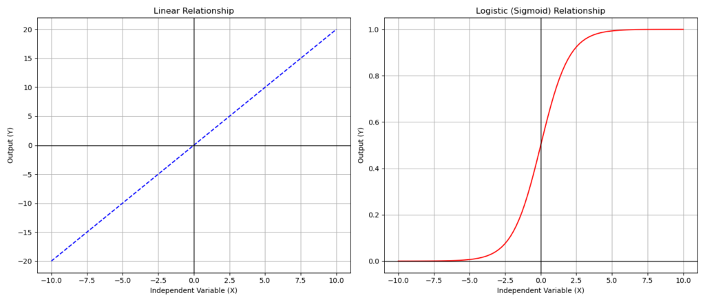
To better understand the difference between linear and logistic regression, consider this: In linear regression, we can determine a specific value for the dependent variable for each combination of independent variables. However, this isn’t possible in logistic regression because the dependent variable can only be 0 or 1. Instead of a straight line, the relationship between variables in logistic regression is represented by a sigmoid curve. This distinction is illustrated in the following figure, which contrasts a linear relationship with a logistic (sigmoid) one.

Odds Ratio
The fundamental concept in logistic regression is that of odds—the ratio between the probability of an event occurring and the probability of it not occurring. In this case, it’s the ratio between the two possible outcomes tracked by the dependent variable. The logit function then calculates the natural logarithm of these odds, transforming the probability scale into a more manageable form for statistical analysis.
![]()
Where:
- p1 and p2 are the probabilities of the event occurring in two different groups
- β is the regression coefficient for the predictor variable
This equation shows that the odds ratio is equal to e raised to the power of the regression coefficient, which is a key interpretation in logistic regression analysis.
Understanding odds ratios is crucial when interpreting regression results.
For example, in a study investigating the impact of regular exercise on heart disease, an odds ratio of 0.6 indicates that people who exercise regularly have 40% lower odds of developing heart disease compared to those who don’t exercise regularly.
For a continuous variable like age in a diabetes study, an odds ratio of 1.05 (for each year increase in age) means that for each one-year increase in age, the odds of developing diabetes increase by 5%.
In a study examining the relationship between gender and depression, an odds ratio of 1.7 (for females compared to males) suggests that females have 1.7 times higher odds of experiencing depression compared to males.
In logistic regression, the dependent variable is typically coded as 0 and 1. The choice of which outcome is assigned 1 is crucial, as the model estimates odds ratios based on this coding.
Conventionally, we code the occurrence of an event or a “success” as 1.
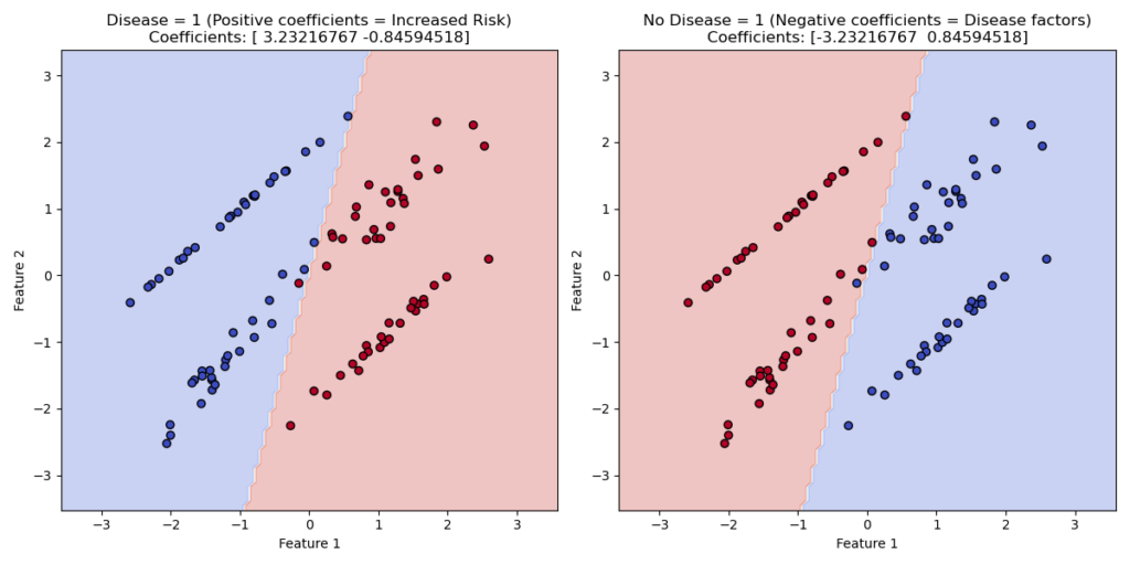
Let’s consider a logistic regression model evaluating the impact of independent variables on disease occurrence. The dependent variable has two possible outcomes: disease or no disease.
If we code “disease” as 1 and “no disease” as 0, the regression coefficients will show how independent variables influence the likelihood of “being sick.” Variables that increase disease risk will have positive coefficients.
Conversely, if we code “no disease” as 1, variables contributing to disease onset will have negative coefficients.
When preparing data, it’s essential to keep these considerations in mind. While the model’s mathematical structure and values remain unchanged, the interpretation of results differs based on the coding choice.

Assumptions
To apply logistic regression techniques, the dependent variable must be binary, while the independent variables can be either continuous or discrete.
In addition to variable types, several other assumptions must be met:
- Independence of observations: The result of one observation must not influence the result of another.
- Linear relationship between independent variables and log-odds: Unlike linear regression, logistic regression doesn’t require a linear relationship between independent and dependent variables. Instead, it requires a linear relationship between the independent variables and the log-odds of the dependent variable (the logarithmic transformation of the success-to-failure ratio). This assumption is crucial.
- Absence of multicollinearity: The independent variables should not be closely correlated with each other.
- Lack of influential outliers: The model should be free from extreme values that could significantly impact the results.
Unlike linear regression, logistic regression doesn’t require homoscedasticity (similar variances) in the data. The regression computation is based on the logarithmic transformation of the odds rather than raw values.
Imbalanced classes can pose a problem. For instance, if the dependent variable can be 0 or 1, and almost all observations are 0, dataset balancing techniques may be necessary to prevent distorted regression results.
Practical guidelines often mention the “rule of 10” and the “rule of 15”:
The “rule of 10” concerns the ratio between observations and rare events. For example, suppose the dependent variable can be 1 or 0, and 1 represents a rare event. In that case, you should have at least 10 cases with a value of 1 for each independent variable in the model.
The “rule of 15” refers to the minimum number of cases needed based on the number of independent variables. For instance, with 5 independent variables, you should have at least 75 cases, regardless of the dependent variable’s distribution.
These empirical rules help prevent model distortions when the number of observations is too low.
Analyzing Output and Results: Coefficient Summary
A logistic regression test yields a wealth of information. The specific output can be customized based on the software used and the researcher’s needs.
At the core of the results lies the “Coefficient Summary.” Let’s examine an example using a hypothetical dataset that explores the relationship between three continuous variables (age, blood pressure, and cholesterol) and the presence or absence of heart disease:
| Variable          | Coef  | Std Err | z      | P>|z| | [95% CI Lower, Upper] |
|-------------------|-------|---------|--------|------|------------------------|
| Age               | 0.05  | 0.02    | 2.5    | 0.01 | [0.01, 0.09]          |
| Blood_Pressure    | 0.03  | 0.01    | 3.0    | 0.002| [0.01, 0.05]          |
| Cholesterol       | 0.01  | 0.003   | 3.3    | 0.0009| [0.004, 0.016]       |
| Constant          | -5.0  | 1.0     | -5.0   | 0.0001| [-7.0, -3.0]         |
The Coef (coefficient) column displays the log-odds ratios for each independent variable. These coefficients represent the change in the log-odds ratio of the dependent variable for each unit increase in the independent variable.
For example, if the coefficient for age is 0.05, each one-year increase in age will result in a 0.05 increase in the log-odds of having heart disease.
To better interpret these coefficients, we can transform the log-odds into odds:
For age, with a log-odds (coefficient) of 0.05, the odds are:
![]()
![]()
This means that for each one-year increase in age, there’s a 5% increase in the odds of heart disease.
Similarly, for blood pressure:
![]()
This indicates that for each unit increase in blood pressure, the odds of cardiovascular disease increase by 3%.
Positive coefficients indicate that an increase in the independent variable corresponds to an increase in the likelihood of the dependent variable occurring. Conversely, negative coefficients signify that an increase in the independent variable decreases this likelihood.
It’s worth noting that some statistical software packages conveniently provide odds ratios alongside the coefficients, simplifying interpretation.
The Standard Error relates to the coefficients and indicates the estimate’s uncertainty. A lower value suggests greater precision.
The z-test is the statistical test of the coefficient. It measures how many standard deviations the coefficient is from zero. A higher absolute z-value indicates stronger evidence against the null hypothesis (that the coefficient is zero).
In SPSS, rather than the z-score, we encounter the Wald test. This test is equivalent to the square of the z-test and follows a chi-square distribution.
The p-value indicates the statistical significance of the variables. A p-value less than 0.05 suggests a statistically significant relationship between the predictor and the outcome.
The 95% confidence intervals show the range of plausible values for the coefficient. If this interval includes zero, it’s unlikely that the predictor has a significant link to the outcome.
The Constant (or intercept) represents the log-odds of having heart disease when all predictors are zero. This serves primarily as a baseline value for the model.


