Normalization, Standardization and Scalers

These are essential operations in the data cleaning process, aimed at preparing data for subsequent analysis or machine learning steps.

Normalization

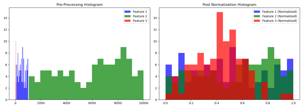
Normalization transforms data to fit within a range of 0 to 1. This ensures that extreme values don’t have a disproportionate impact.

Normalization is achieved using the following formula:

X_norm = normalized value; X_origin = original value ; X_min = minimum value and X_max = maximum values in the dataset.

Standardization

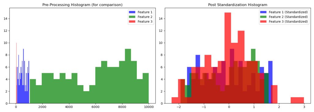
Standardization transforms data to have a mean of 0 and a standard deviation of 1.

The formula is:

X_stand = the standardized value; x = original value; μ = mean of the distribution; σ = standard deviation of the distribution

Normalization is typically used for data with an arbitrary or non-normal distribution, whereas standardization is more suitable for data that follows a normal or near-normal distribution.

Outliers significantly influence normalization by modifying the minimum and maximum values used for transformation. In contrast, standardization is less directly affected by outliers. However, they can still impact the mean and standard deviation in standardization, albeit to a lesser degree than normalization.

Normalization is useful when comparing measurements with different scales (for example, weight and height), making them compatible with each other.

Standardization is useful in algorithms like logistic regression or PCA (Principal Component Analysis) because the scale of the data affects the results in these cases.

In many machine learning applications, these processes are called “scaling.” This term refers to modifying the scale or range of data using a specific mathematical operation.

Data scaling can occur in two main ways:

1. Relative scaling: In normalization, data is modified to fit within a specific range (typically between 0 and 1). This process effectively “compresses” or “expands” the data to fit within the desired range.
2. Statistical scaling: In standardization, the distribution of the data is modified to have specific statistical properties, such as a mean of 0 and a standard deviation of 1.

The Python library scikit-learn offers various Scalers that can be applied during the data preprocessing stage.

MinMaxScaler (Normalization): Transforms data to fit within a specific range, typically 0 to 1.

StandardScaler (Standardization): Modifies data to have a distribution with a mean of 0 and a standard deviation of 1.

MaxAbsScaler: Scales data so that the maximum absolute value is 1. Useful for preserving the sign of values and their ratios, especially with negative numbers.

RobustScaler: Uses median and interquartile range (IQR) for scaling, making it less sensitive to outliers than other scalers.

QuantileTransformer: Transforms data to have a uniform or Gaussian distribution.

PowerTransformer: Applies a transformation to make data more closely resemble a normal distribution.

Normalizer: Unlike column-based scalers, this applies to dataset rows. It transforms each row to have a norm of 1, preserving the direction of data vectors—crucial in NLP and neural networks.

To illustrate the processes of normalization and standardization in Python, let’s create three variables (features) for an imaginary dataset:

1. One containing values between 100 and 1,000
2. Another with values between 1,000 and 10,000
3. A third with a normal distribution (mean of 50, standard deviation of 10)

We’ll create graphs after applying normalization (using MinMaxScaler) and standardization (using StandardScaler) to these variables.

import numpy as np
import pandas as pd
import matplotlib.pyplot as plt
from sklearn.preprocessing import MinMaxScaler, StandardScaler

# Create a sample dataset
np.random.seed(42)
data = {
    'Feature_1': np.random.randint(100, 1000, 100),
    'Feature_2': np.random.randint(1000, 10000, 100),
    'Feature_3': np.random.normal(50, 10, 100)  # Normally distributed
}

df = pd.DataFrame(data)

# Create pre-processing data visualizations
fig, ax = plt.subplots(1, 2, figsize=(14, 5))

ax[0].hist(df['Feature_1'], bins=20, color='b', alpha=0.7, label='Feature 1')
ax[0].hist(df['Feature_2'], bins=20, color='g', alpha=0.7, label='Feature 2')
ax[0].hist(df['Feature_3'], bins=20, color='r', alpha=0.7, label='Feature 3')
ax[0].set_title('Pre-Processing Histogram')
ax[0].legend()

# Normalization (Min-Max Scaling)
scaler = MinMaxScaler()
normalized_data = scaler.fit_transform(df)

# Standardization (Z-score)
std_scaler = StandardScaler()
standardized_data = std_scaler.fit_transform(df)

# Post Normalization Visualization
ax[1].hist(normalized_data[:, 0], bins=20, color='b', alpha=0.7, label='Feature 1 (Normalized)')
ax[1].hist(normalized_data[:, 1], bins=20, color='g', alpha=0.7, label='Feature 2 (Normalized)')
ax[1].hist(normalized_data[:, 2], bins=20, color='r', alpha=0.7, label='Feature 3 (Normalized)')
ax[1].set_title('Post Normalization Histogram')
ax[1].legend()

plt.tight_layout()
plt.show()

# Create plots for Standardization
fig, ax = plt.subplots(1, 2, figsize=(14, 5))

# Pre-processing visualization again for comparison
ax[0].hist(df['Feature_1'], bins=20, color='b', alpha=0.7, label='Feature 1')
ax[0].hist(df['Feature_2'], bins=20, color='g', alpha=0.7, label='Feature 2')
ax[0].hist(df['Feature_3'], bins=20, color='r', alpha=0.7, label='Feature 3')
ax[0].set_title('Pre-Processing Histogram (for comparison)')
ax[0].legend()

# Post Standardization Visualization
ax[1].hist(standardized_data[:, 0], bins=20, color='b', alpha=0.7, label='Feature 1 (Standardized)')
ax[1].hist(standardized_data[:, 1], bins=20, color='g', alpha=0.7, label='Feature 2 (Standardized)')
ax[1].hist(standardized_data[:, 2], bins=20, color='r', alpha=0.7, label='Feature 3 (Standardized)')
ax[1].set_title('Post Standardization Histogram')
ax[1].legend()

plt.tight_layout()
plt.show()

The graphs generated by the code visually demonstrate the outcomes of normalization and standardization: