In a previous blog post, we explored how to read the content of a DICOM file, including its numerous tags. These tags provide insights into the study type, characteristics, and all relevant patient and study information.

Now, we’ll focus on the most crucial tag—the one containing the images. A typical study can include anywhere from a few to several hundred DICOM files, usually identifiable by their .dcm extension.

For our practice, we’ll open a single .dcm file containing a frontal projection chest X-ray.

Environment Setup

Before we begin, it’s essential to install some key libraries. Due to dependency issues, it’s best to create a dedicated environment for running Python with these libraries. In our environment, we’ve installed numpy, pandas, and matplotlib—common libraries for data management and visualization—as well as the pydicom library discussed in our previous post.

For this specific task, we’ve also installed these additional libraries:

scipy: An open-source library for scientific computing in Python, based on numpy. It’s particularly useful for applying image transformation filters.

opencv (cv2): The Open Source Computer Vision Library, which uses machine learning for computer vision tasks. It provides various tools for image processing. In Python, you can access it through the cv2 module.

pylibjpeg, pylibjpeg-libjpeg, and gdcm: These libraries are necessary for working with and processing DICOM files.

Our radiographic image is located at IMAGES\01\00001.dcm on a diagnostic CD. It contains a frontal projection chest X-ray. The same directory also includes file 00002.dcm, which contains the lateral projection—we won’t be using this for now.

Loading the image

First, let’s import the necessary libraries:

import pydicom
import matplotlib.pyplot as plt
import numpy as np

Now, we’ll locate our .dcm file and load the dataset into the dicom_data variable.

The image data in dicom_data is stored in the pixel_array attribute, which we’ll assign to the image variable. This creates a numpy array of rows and columns containing the pixel data that forms the image.

# Specify the path to the DICOM file
dicom_path = "C:\\Dicom\\RX\\IMAGES\\01\\00001"

# Read the DICOM file
dicom_data = pydicom.dcmread(dicom_path)

# Extract the image from the DICOM dataset
image = dicom_data.pixel_array:

Let’s extract some key information about our image: its data type, dimensions in pixels, and the range of possible pixel values:

# Information about the array
print("Pixel data type:", image.dtype)
print("Image dimensions:", image.shape)
print("Maximum pixel value:", np.max(image))
print("Minimum pixel value:", np.min(image))

Pixel data type: uint16 Image

dimensions: (2400, 2880)

Maximum pixel value: 4095

Minimum pixel value: 0

Our image has dimensions of 2400 x 2880 pixels, with each pixel capable of holding a value from 0 to 4095.

The pixel data type indicates a bit depth of 16 unsigned bits (u) per pixel, allowing for 2^16 = 65,536 grayscale values (opacity and brightness) ranging from 0 to 65,535. In contrast, an 8-bit image has a lower depth, with each value on the scale ranging from 0 to 255 (2^8 = 256 values).

However, it’s worth noting that while the data type allows for up to 65,535 values, the actual image in this case only uses values from 0 to 4095. This suggests that the image is effectively using 12 bits of information (2^12 = 4096 possible values), even though it’s stored in a 16-bit format.

Medical images are typically stored in 12- or 16-bit formats. The lowest values (0) correspond to darker areas in the image.

We can visualize the image using matplotlib:

# Display the image
plt.imshow(image, cmap="gray")
plt.axis("off")  # Hide axes for a clean visualization
plt.show()

The resulting image will be displayed as follows:

Out of curiosity, let’s extract the values from a small 10×10 pixel area of the image, read the stored values, and reconstruct them based on the grayscale.

# Define the starting position for the square (you can modify it based on your needs)
start_x, start_y = 100, 100  # For example, the top-left pixel of the square

# Extract a 10x10 pixel square from the resized frontal image
square = image[start_y:start_y+10, start_x:start_x+10]

# Display the numerical values of the pixels
fig, axes = plt.subplots(1, 2, figsize=(12, 6))

# First grid: numerical pixel values
axes[0].imshow(square, cmap="gray")
for i in range(10):
    for j in range(10):
        # Insert the pixel value at the center of the cell
        axes[0].text(j, i, int(square[i, j]), ha="center", va="center", color="red", fontsize=10)
axes[0].set_title("Pixel Values")
axes[0].axis("off")  # Remove axes for a clean visualization

# Second grid: grayscale
axes[1].imshow(square, cmap="gray")
axes[1].set_title("Grayscale")
axes[1].axis("off")

# Optimize the layout
plt.tight_layout()
plt.show()

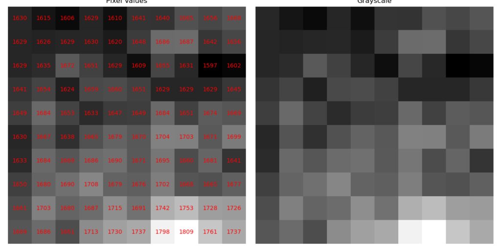
Various operations can be performed on the pixel matrix that composes the image. Let’s explore a few of them.

Normalization

When the grayscale range is extensive (in our case, from 0 to 65,535), it’s often beneficial to normalize it to a scale of 0 to 255. This process can enhance the visibility of details perchè con valori di intensità molto distanti potrebbero essere non distinguibili.

When the grayscale range is extensive (in our case, from 0 to 65,535), it’s often beneficial to normalize it to a scale of 0 to 255. This process can enhance the visibility of details, as intensity values that are very far apart might otherwise be indistinguishable to the human eye.

# Normalization between 0 and 255
image_normalized = (image - np.min(image)) / (np.max(image) - np.min(image)) * 255
image_normalized = image_normalized.astype(np.uint8)

# Display the normalized image
plt.imshow(image_normalized, cmap="gray")
plt.title("Normalized Image")
plt.axis("off")
plt.show()

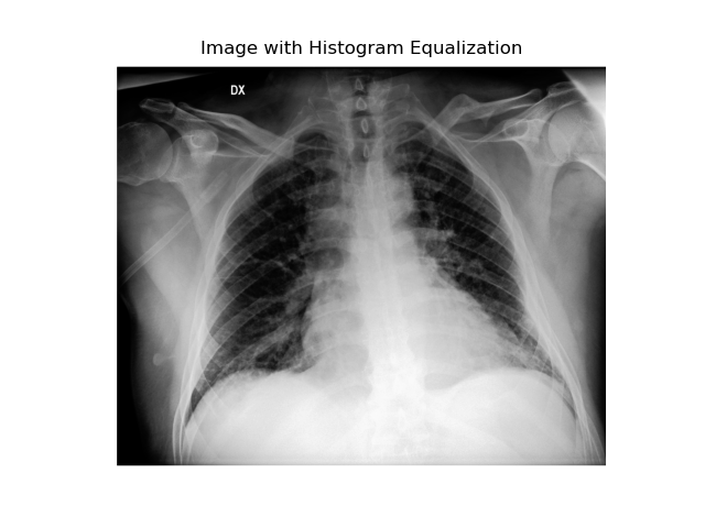
Equalization

This technique adjusts pixel values to better distribute intensities across the image. It’s particularly useful for radiographic images as it enhances the visibility of structures that are otherwise difficult to perceive.

To perform equalization, we’ll use the cv2 library:

import cv2

# Histogram equalization with OpenCV
image_equalized = cv2.equalizeHist(image_normalized)
plt.imshow(image_equalized, cmap="gray")
plt.title("Image with Histogram Equalization")
plt.axis("off")
plt.show()

Smoothing or Gaussian Filter

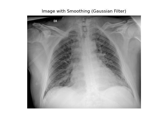
The Gaussian filter averages nearby pixels to reduce sudden value variations and noise. As a result, images appear less detailed but more uniform.

You can import the Gaussian filter from scipy.

from scipy.ndimage import gaussian_filter

# Apply a Gaussian filter to reduce noise
image_smoothed = gaussian_filter(image_normalized, sigma=1)

# Display the image with smoothing
plt.imshow(image_smoothed, cmap="gray")
plt.title("Image with Smoothing (Gaussian Filter)")
plt.axis("off")
plt.show()

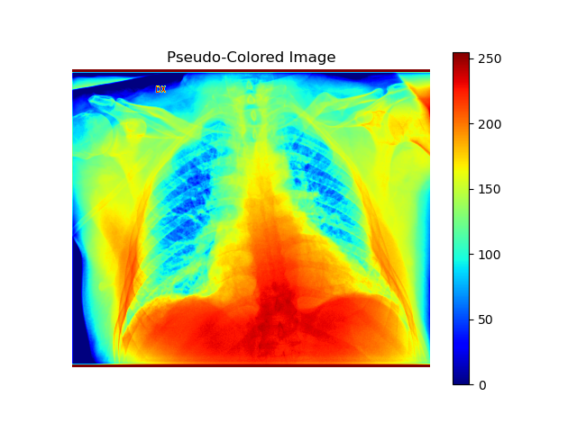
Pseudocoloring

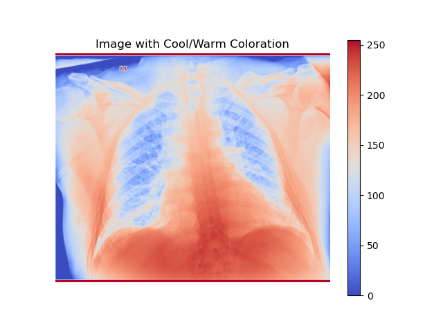
Pseudocoloring applies filters to colorize areas in grayscale images, enhancing visual analysis. For instance, the “jet” filter assigns blue to low intensities and red to high intensities, making different regions more distinguishable.

# Apply a "jet" color map for pseudo-coloring
plt.imshow(image_normalized, cmap="jet")
plt.title("Pseudo-Colored Image")
plt.axis("off")
plt.colorbar()  # Add a color bar for reference
plt.show()

Another color scale option is the cool/warm scale:

plt.imshow(image_normalized, cmap="coolwarm")
plt.title("Image with Cool/Warm Coloration")
plt.axis("off")
plt.colorbar()
plt.show()

Thresholding

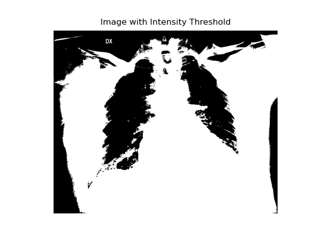
The image is converted to binary, with pixels below a certain threshold becoming black and those above turning white. This process highlights high-density elements like bones in an X-ray.

threshold_value = 128  # Example threshold, to be adapted to the image
image_thresholded = (image_normalized > threshold_value) * 255

plt.imshow(image_thresholded, cmap="gray")
plt.title("Image with Intensity Threshold")
plt.axis("off")
plt.show()

Edge Detection (Canny)

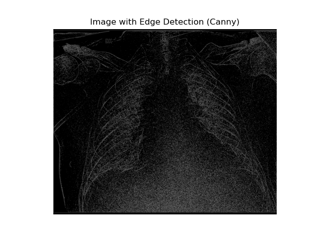
The Canny edge detection algorithm identifies edges in an image based on intensity gradients. It uses two threshold values to determine which edges to keep.

# Apply edge detection using OpenCV's Canny method
edges = cv2.Canny(image_normalized, threshold1=30, threshold2=34)

# Display the detected edges
plt.imshow(edges, cmap="gray")
plt.title("Image with Edge Detection (Canny)")
plt.axis("off")
plt.show()

With the pixel matrix that composes an image at our disposal, we have a wide array of manipulation techniques to enhance its visualization. These techniques allow us to extract more information, highlight specific features, or improve the overall clarity of the image.

In many medical imaging scenarios, we often encounter multiple images of the same patient and anatomical region. This presents exciting opportunities beyond single-image manipulation. We can use these multiple images to reconstruct three-dimensional volumes, providing a more comprehensive view of the anatomy. Additionally, we can create dynamic sequences or moving images, which can be particularly useful for studying physiological processes or changes over time.

These advanced processing techniques, such as volume reconstruction and dynamic imaging, open up new possibilities for diagnosis, treatment planning, and medical research. They allow healthcare professionals to gain deeper insights into patient anatomy and physiology, potentially leading to more accurate diagnoses and improved patient care