Repeated measures ANOVA is used when multiple measurements are taken on the same experimental units. For instance, a parameter like blood pressure might be measured on the same person at different times or under varying conditions.
This approach doesn’t meet the independence assumption, unlike one-way or multi-way ANOVA. By definition, it’s the same subject receiving multiple observations or measurements.
For the repeated measures ANOVA test to be applicable, certain conditions must be met:
- Normality: The measurements of the dependent variable must be normally distributed at each time point or condition.
- Independence: The experimental units (subjects) must be independent, while the measurements are not, as they’re performed on the same subjects.
- Homogeneity of variance: The variances between groups must be similar.
- Sphericity: The differences between measurements across groups must have constant variability. This is crucial, as violating this assumption may distort the test results.
In practice, the choice between repeated measures ANOVA and paired t-test depends on the number of conditions or time points. For up to two conditions or measurement times, a paired t-test is appropriate. For more than two, repeated measures ANOVA is indicated.
Repeated measures ANOVA can still be applied when there are only two conditions or measurement times. However, its result will be identical to the t-test, which is simpler and easier to interpret.
Sphericity and Corrections for Sphericity
A key assumption for correctly analyzing data with repeated measures ANOVA is sphericity.
The concept of sphericity involves the condition where the variances of the differences across the various measures from different groups are equal. This means that the differences in measurements between the groups are consistent in their variability, which is critical when analyzing repeated measures in ANOVA.

The graph above illustrates the concept of sphericity: the variances between conditions differ significantly, indicating a violation of the sphericity assumption. This inconsistency in differences between conditions could lead to distorted results in traditional ANOVA if left uncorrected.
The Mauchly test is commonly used to determine whether the assumption of sphericity is upheld. The null hypothesis states that the variance of differences between levels is equal. Therefore, a significant test value (p < 0.05) indicates a violation of sphericity.
The verification process for ensuring sphericity is crucial because, in instances where this assumption is not met, the calculated F-statistic becomes disproportionately large. This situation subsequently results in an increased likelihood of committing a Type I error, characterized by an elevated rate of false positives in the statistical analysis.
When sphericity is present, the ANOVA test is valid. However, if Mauchly’s test doesn’t confirm sphericity, researchers can take two approaches:
- Apply sphericity corrections: This process involves adjusting the degrees of freedom associated with the F test by applying a specific factor referred to as epsilon. The most common corrections are: GGe = Greenhouse-Geisser epsilon HFe = Huynh-Feldt epsilon In both cases, the degrees of freedom are adjusted and then multiplied by epsilon to obtain the adjusted p-value. Although the two tests usually yield similar results, GGe is typically applied to cases with moderate to severe sphericity violations, while HFe is used for less severe violations (with epsilon > 0.75).
- Use multivariate tests as an alternative to traditional repeated measures ANOVA
Multivariate Test
.Several multivariate tests can be performed when the lack of sphericity compromises the reliability of the repeated measures ANOVA test.
These include:
- Pillai’s Trace: Robust and tolerant of normality and sphericity violations, but with lower statistical power (less ability to detect significant differences)
- Wilk’s Lambda: One of the most commonly used and reported multivariate tests, though less robust when assumptions are violated
- Hotelling’s Trace: More powerful but less robust than Pillai’s Trace
- Roy’s Largest Root: More sensitive but less robust, useful when one group shows a dominant difference compared to others
While not mathematically complementary, Pillai’s Trace and Wilk’s Lambda are interpretatively opposite. Pillai’s Trace indicates the variance explained by condition differences, while Wilk’s Lambda shows the variance not explained by these differences. As Pillai’s Trace increases, Wilk’s Lambda decreases. Both tests, when significant, indicate differences between conditions.
Model Type
When dealing with multiple independent variables, it is crucial to verify the model structure. A full-factorial model incorporates all independent variables and their interactions, providing a comprehensive analysis of the data. This approach allows for the examination of main effects as well as potential interaction effects between variables. However, it’s important to note that a full-factorial model may not always be the most appropriate choice. Depending on the research questions and the nature of the data, we might opt for a different model structure. For instance, we could choose a main effects model that only considers the individual effects of each variable without interactions, or a hierarchical model that introduces variables in a specific order based on theoretical considerations. The selection of the most suitable model depends on various factors, including the study design, hypotheses, and the complexity of the relationships between variables.
Types of Sum of Squares
An additional factor to consider when calculating repeated measures ANOVA is the type of sum of squares, a topic we’ve explored in a previous post.
Contrasts
A contrast is a specific comparison between group means in a statistical analysis. It’s a way to test targeted hypotheses about how groups differ from each other,
There are several ways to compare group means:
- Simple Contrasts: Compare one group to another (e.g., group A versus group B).
- Helmert Contrasts: Compare one group to the mean of subsequent groups.
- Difference Contrast: Compare each group to the previous one in a sequence.
- Deviation Contrast: Compare each group to the overall mean of all groups.
Results of the Repeated Measures ANOVA Test:
The repeated measures ANOVA test calculates the F statistic, which compares two estimated variances: the variance between groups or conditions (reflecting systematic differences) and the variance within groups or conditions (reflecting random variability). A high F value suggests that the variability between groups exceeds the variability within groups, indicating potentially significant differences.
Typically, the test results include:
- Main effect of the within-subjects factor: Determines if there are differences between repeated measures (e.g., if means differ across conditions or times).
- Interaction effect: Assesses if there’s a significant interaction between the within-subjects factor and other factors (such as treatment groups, if present).
- F statistic: Indicates whether the observed differences between conditions are statistically significant.
- P-value: Provides the probability that the observed differences are due to chance.
- Standard error values and confidence intervals: Offer information on the precision of the mean estimates.
Post-hoc Analysis
In repeated measures ANOVA, as with one-way ANOVA, a statistically significant result prompts further investigation to pinpoint which specific groups drive the observed differences. This deeper exploration is achieved through post-hoc analysis, a method we’ve previously discussed for one-way ANOVA.
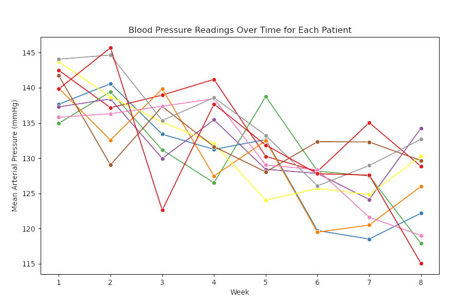
Here’s an example of a statistical analysis using repeated measures ANOVA. We’ll create a fictional dataset simulating the administration of an antihypertensive drug to 10 patients over two months, measuring their mean arterial pressure weekly.
# Importing necessary libraries for the analysis
import pandas as pd
import numpy as np
import matplotlib.pyplot as plt
import seaborn as sns
from statsmodels.stats.anova import AnovaRM

# Set random seed for reproducibility
np.random.seed(42)

# Parameters for the dataset
n_patients = 10
n_weeks = 8
base_bp = 140  # Baseline blood pressure for patients
treatment_effect = np.linspace(0, -15, n_weeks)  # Gradual treatment effect (reduction in BP over time)

# Creating a DataFrame with PatientID, Week, and BloodPressure
data = pd.DataFrame({
    'PatientID': np.repeat(np.arange(1, n_patients + 1), n_weeks),
    'Week': np.tile(np.arange(1, n_weeks + 1), n_patients),
    'BloodPressure': np.random.normal(base_bp, 5, n_patients * n_weeks) + np.tile(treatment_effect, n_patients)
})

# Visualizing the data
plt.figure(figsize=(10, 6))
sns.lineplot(x='Week', y='BloodPressure', hue='PatientID', marker='o', data=data, palette='Set1')
plt.title('Blood Pressure Readings Over Time for Each Patient')
plt.ylabel('Mean Arterial Pressure (mmHg)')
plt.xlabel('Week')
plt.legend(title='Patient ID', bbox_to_anchor=(1.05, 1), loc='upper left')
plt.show()
The graph clearly demonstrates a downward trend in blood pressure over time. Let’s now conduct a repeated measures ANOVA to analyze this trend statistically.
# Performing Repeated Measures ANOVA
rm_anova = AnovaRM(data, 'BloodPressure', 'PatientID', within=['Week'])
rm_results = rm_anova.fit()

rm_results.summary()
The repeated measures ANOVA results are as follows:
- F-statistic: 13.95
- Degrees of Freedom (Num DF): 7 (for the 8 weeks)
- Degrees of Freedom (Den DF): 63 (within-patient variability)
- p-value: < 0.0001
The p-value is highly significant, indicating a statistically significant difference in blood pressure readings across the weeks.
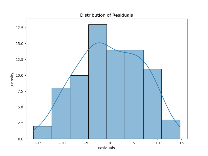
Next, we test the assumptions, starting with checking residuals for normality.
# Calculate residuals for each patient
data['Residuals'] = data.groupby('PatientID')['BloodPressure'].transform(lambda x: x - x.mean())

# Plotting the residuals
plt.figure(figsize=(8, 6))
sns.histplot(data['Residuals'], kde=True)
plt.title('Distribution of Residuals')
plt.xlabel('Residuals')
plt.ylabel('Density')
plt.show()

We conduct post-hoc analysis to pinpoint which groups are responsible for the observed statistical differences:
from statsmodels.stats.multicomp import pairwise_tukeyhsd

# Tukey's HSD (adapted for pairwise comparisons using this method for repeated measures)
# Flatten the data so that Tukey's test can be applied (Note: Tukey's test is more suited for between-subjects)
tukey = pairwise_tukeyhsd(endog=data['BloodPressure'], groups=data['Week'], alpha=0.05)

# Display Tukey's HSD results
tukey_results = tukey.summary()

tukey_results
Based on our analysis, we can conclude the following:
- Significant decreases in blood pressure are evident when comparing Week 1 with Weeks 5 and 6. This suggests that the antihypertensive therapy had a substantial effect during these periods.
- Other comparisons, such as Week 1 vs Week 2, showed no significant differences, implying that the treatment effect was more gradual initially.
These findings indicate that the blood pressure reduction became more pronounced in the later weeks of the treatment, highlighting the cumulative effect of the therapy over time.


