When setting up a repeated measures ANOVA test in SPSS, the dialog box for the model has “Type 3 sum of squares” selected by default. By exploring the window further, you’ll find that you can also choose Type 1, Type 2, or Type 4 sum of squares.
How many types of Sums of Squares are there, and when should you use each one?
This issue is relevant because choosing one type over another can significantly affect the analysis results, particularly with unbalanced data or when certain assumptions are violated.
Let’s examine the different types.
The examples will be based on a hypothetical experiment with two factors: Factor A (with 2 levels: A1 and A2) and Factor B (with 2 levels: B1 and B2). Let’s assume we also have an interaction between A and B (A x B).
Type 1 SS
In Type 1 Sum of Squares, the calculation process follows a sequential order, which means that each effect is evaluated conditionally based on the effects that precede it in the model. This approach allows for a hierarchical assessment of the factors and their interactions.
The sequential nature of Type 1 SS results in the following order of calculations:
- SS(A) = Variation explained by factor A This represents the amount of variability in the dependent variable that can be attributed solely to factor A, without considering any other factors or interactions.
- SS(B|A) = Variation explained by factor B after accounting for factor A This calculation determines the additional variability explained by factor B, but only after the effects of factor A have been taken into account. It essentially measures the unique contribution of factor B beyond what has already been explained by factor A.
- SS(AB|A,B) = Variation explained by the interaction of AxB after considering both A and B This final step evaluates the amount of variability that can be attributed to the interaction between factors A and B, but only after the individual effects of both A and B have been accounted for. It represents the synergistic or antagonistic effects that occur when the two factors are combined.
It’s important to note that the order in which factors are entered into the model can significantly impact the results of Type 1 SS, especially in cases of unbalanced designs or when there are correlations between the predictors.
Type 2 SS
Type 2 Sum of Squares (SS) evaluates each effect independently for main effects, without considering interactions. This approach provides a more balanced assessment of each factor’s contribution to the overall variability in the data.
The calculation process for Type 2 SS follows a specific order, which allows for a comprehensive analysis of the main effects while maintaining the integrity of each factor’s individual impact. The sequence of calculations is as follows:
- SS(A|B): This step calculates the variation explained by Factor A, while taking into account the presence of Factor B. It’s important to note that this calculation does not consider any potential interaction between the two factors. This allows for an isolated assessment of Factor A’s main effect, controlling for the influence of Factor B.
- SS(B|A): Similarly, this calculation determines the variation explained by Factor B, while accounting for the presence of Factor A. Again, the interaction between the factors is not considered at this stage. This step provides insight into the unique contribution of Factor B to the overall variability, independent of Factor A’s influence.
- SS(AB|A, B): The final step in Type 2 SS involves calculating the variation explained by the interaction between Factors A and B, after both main effects have been accounted for. This calculation is identical to the one used in Type I SS for the interaction term. It reveals any additional variability that can be attributed to the combined effect of the two factors, beyond their individual main effects.
Type 2 SS is most useful when the primary focus is on main effects, and interactions are either not of interest or absent. This approach is particularly effective in balanced experimental designs.
Type 3 SS
Type III sum of squares evaluates each main effect and interaction while controlling for all other effects (both main effects and interactions). This approach provides a comprehensive assessment of each factor’s unique contribution to the model.
The calculation process for Type 3 Sum of Squares follows a specific order, ensuring that each effect is evaluated while controlling for all other effects in the model. This comprehensive approach allows for a more nuanced understanding of each factor’s unique contribution to the overall variability. The sequence of calculations is as follows:
- SS(A|B, AB): This step calculates the variation explained by Factor A, while simultaneously controlling for both Factor B and the interaction between A and B (AB). By doing so, we isolate the unique effect of Factor A, independent of any influence from Factor B or their interaction. This provides a pure measure of Factor A’s contribution to the model.
- SS(B|A, AB): Similarly, this calculation determines the variation explained by Factor B, while controlling for Factor A and the AB interaction. This approach allows us to assess the unique impact of Factor B on the dependent variable, separate from any effects of Factor A or their interaction. It offers insight into Factor B’s individual contribution to the overall variability in the data.
- SS(AB|A, B): The final step involves calculating the variation explained by the interaction between Factors A and B, while controlling for both main effects. This calculation reveals any additional variability that can be attributed to the synergistic or antagonistic effects of the two factors combined, beyond what can be explained by their individual main effects. It provides crucial information about how the factors work together to influence the dependent variable.
Type 3 SS is particularly valuable in complex experimental designs, especially when dealing with unbalanced data or when interactions between factors are of primary interest. By controlling for all other effects, it provides a robust and unbiased assessment of each factor’s unique contribution to the model, regardless of the order in which the factors are entered into the analysis.
This method is widely used across many statistical software packages and is the default option in SPSS.
Type 4 SS
Type 4 sums of squares are designed to handle cases with missing data or particularly complex and unbalanced designs. They account for empty cells (missing data), enabling a more precise analysis in these challenging situations.
Type 5 SS
Type 5 SS is less common and is specifically used for certain experimental designs, particularly those involving covariates or mixed models.
Interaction Between Factors
When conducting a repeated measures ANOVA test with two or more factors, we must consider not only the effect of individual factors on the dependent variable but also the interactions between them.
If there’s an interaction between two factors, A and B, the final effect isn’t simply the sum of A’s effect and B’s effect. Instead, it includes their interaction as well.
Consider testing a drug’s effectiveness in treating hypertension (Factor A: A1 drug present, A2 drug absent) while also putting patients on a diet (Factor B: B1 diet with high protein present, B2 diet absent). The final effect on blood pressure won’t just be the combined effect of the drug and diet. It will also depend on how they interact. For instance, the drug’s effect might be enhanced when combined with the diet and diminished without it.
When interaction occurs, it complicates the attribution of effects to individual factors and makes interpreting the phenomenon more challenging. Moreover, the interaction itself may become the study’s primary focus, often proving more intriguing than the effects of individual factors alone.
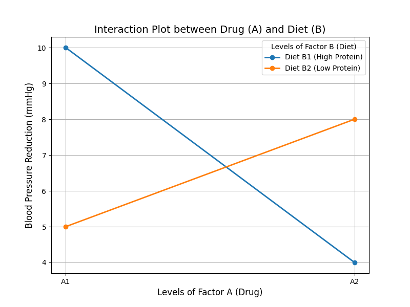
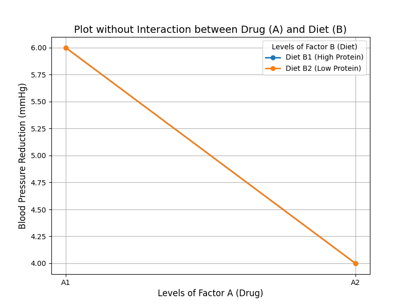
Let’s visually represent how factors A (drug) and B (diet) affect blood pressure values, both with and without interaction.
import matplotlib.pyplot as plt
import numpy as np

# Hypothetical data for interaction plot
# Factor A with two levels: A1 and A2
# Factor B with two levels: B1 and B2

# Levels of Factor A (e.g., Drug: Present (A1) and Absent (A2))
A_levels = ['A1', 'A2']

# Example with interaction between factors
# Blood pressure reduction for different levels
# Effect of the drug (Factor A) at different levels of diet (Factor B)
reduction_B1_interaction = [10, 4]  # Effect of A1 and A2 with Diet B1 (High Protein)
reduction_B2_interaction = [5, 8]   # Effect of A1 and A2 with Diet B2 (Low Protein)

# Plotting the interaction graph
plt.figure(figsize=(8, 6))

# Plot lines for different levels of Factor B
plt.plot(A_levels, reduction_B1_interaction, marker='o', label='Diet B1 (High Protein)', linestyle='-', linewidth=2)
plt.plot(A_levels, reduction_B2_interaction, marker='o', label='Diet B2 (Low Protein)', linestyle='-', linewidth=2)

# Adding labels and title
plt.xlabel('Levels of Factor A (Drug)', fontsize=12)
plt.ylabel('Blood Pressure Reduction (mmHg)', fontsize=12)
plt.title('Interaction Plot between Drug (A) and Diet (B)', fontsize=14)

# Adding a legend
plt.legend(title='Levels of Factor B (Diet)', fontsize=10)

# Display the plot
plt.grid(True)
plt.show()

# Example without interaction between factors
# Blood pressure reduction for different levels
# Here, the effect of the drug (Factor A) is consistent across both diets (Factor B)
reduction_B1_no_interaction = [6, 4]  # Effect of A1 and A2 with Diet B1 (High Protein)
reduction_B2_no_interaction = [6, 4]  # Effect of A1 and A2 with Diet B2 (Low Protein)

# Plotting the non-interaction graph
plt.figure(figsize=(8, 6))

# Plot lines for different levels of Factor B
plt.plot(A_levels, reduction_B1_no_interaction, marker='o', label='Diet B1 (High Protein)', linestyle='-', linewidth=2)
plt.plot(A_levels, reduction_B2_no_interaction, marker='o', label='Diet B2 (Low Protein)', linestyle='-', linewidth=2)

# Adding labels and title
plt.xlabel('Levels of Factor A (Drug)', fontsize=12)
plt.ylabel('Blood Pressure Reduction (mmHg)', fontsize=12)
plt.title('Plot without Interaction between Drug (A) and Diet (B)', fontsize=14)

# Adding a legend
plt.legend(title='Levels of Factor B (Diet)', fontsize=10)

# Display the plot
plt.grid(True)
plt.show()

Interaction Plot: This graph illustrates the interaction between the drug (Factor A) and diet (Factor B). The drug’s effect on blood pressure reduction varies depending on the diet type. With Diet B1 (High Protein), the reduction is greater when the drug is present (A1) compared to when it’s absent (A2). Conversely, for Diet B2 (Low Protein), this pattern reverses. This clear reversal demonstrates a significant interaction between the two factors.

Plot without Interaction: This graph shows no interaction between the drug and diet. The drug’s effect (A1 vs. A2) remains consistent across both diet types (B1 and B2). The parallel lines indicate that the diet doesn’t influence how the drug affects blood pressure reduction.
